How to sample from any^* Probability Distribution [md]

Introduction

One of the reasons computers came to be is for tasks that require an absurd amount of repetition. Tasks such as sorting millions of rows of a database, or intersection-testing¹ billions of rays to generate renders Figure-1. A lot of these tasks also benefit from some amount of randomization, some amount of general “iffy”-ness.

I want to focus on this randomness. What does it mean for something to be random? Is it complete chaos - arbitrary? Technically speaking, yes, but it’s not necessarily what we intend. So, usually, there is some reasoning behind the randomness we want. There are many ways this can be controlled.

Here we look at using probability distributions to guide our randomness.

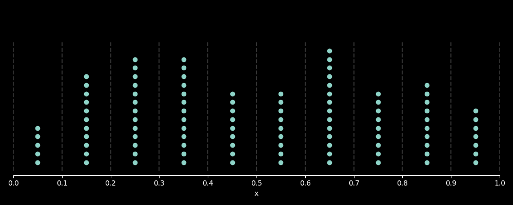
Imagine a scenario where we want to distribute points along a number line, and collect them into 10 buckets. Let’s look at 2 ways we can do this -

1. We distribute the points across the number line with equal probability, i.e., following the pdf $p(x) = 1$ Figure-2

2. We distribute the points following an arbitrary pdf, here we follow the pdf $p(x) = 2x$ Figure-3.

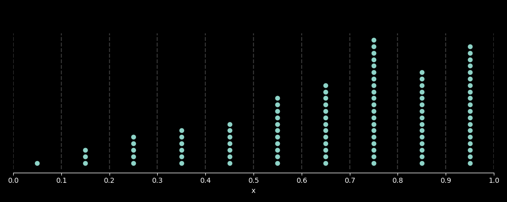
We can see that simply selecting the pdf the outcomes look quite different. Here, I intend to look at one particular method for generating samples that follow a pdf.

The Method

For the common cases such as uniformly distributed samples (probability everywhere is the same), or normally distributed samples (samples that follow the gaussian distribution), usually the standard libraries have functions to generate these samples that follow tried and tested methods that are much beyond the scope of what is discussed here. In fact, the method I am about to discuss hinges on the fact that we can obtain a uniformly distributed variable $\xi_i$ from (usually) the standard library².

So, rather than talking about the common distributions, lets look at a generic probability distribution that follows the probability density function (or probability mass function in the discrete case) , $p(x)$.

So, here is the method. Given a generic distribution $p(x)$. To generate samples $X_i$ that follow the pdf, we -

1. Obtain the cumulative distribution functions (CDF) by integrating the PDF - $P(x) = \int_{0}^{x} p(x') dx'$
2. Compute the inverse of this CDF $P^{-1}(x)$
3. Get the sample $\xi_i$ that is uniformly distributed in $[0, 1]$
4. Finally, map $\xi_i \rArr X_i$ by $X_i = P^{-1}(\xi_i)$

As we can see, the one caveat of this algorithm is that the the function must be integrable. This might disqualify it from certain use cases, such as following a normal distribution, but there exist other methods for sampling from such popular distributions ³.

A few examples

A Continous PDF

Now I find this algorithm to be really quite elegant, because of how obvious it seems when we visualize it. But for that, first we look at a few examples of this algorithm. Let’s say we want to sample the distribution (Figure-4)

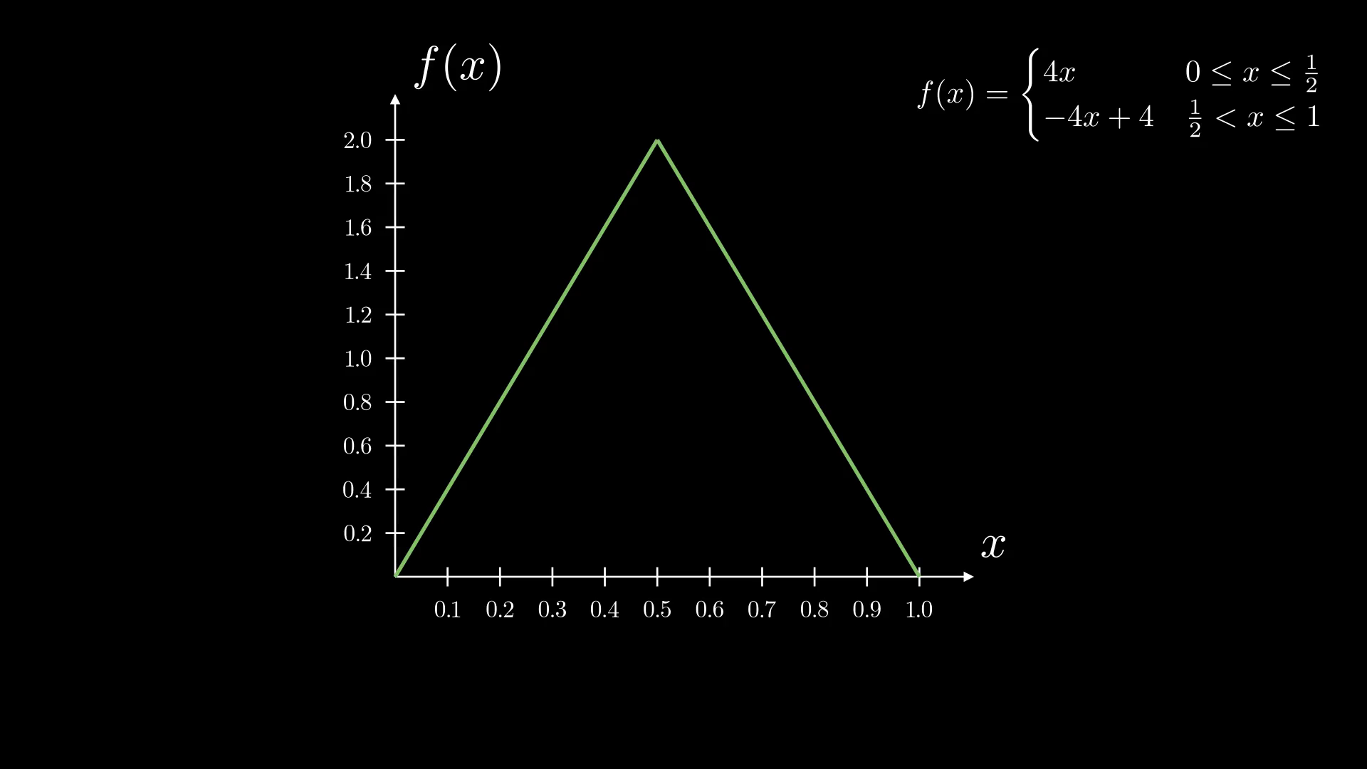
So, following the 4 steps we get -

1. Finding the CDF (Figure-5)

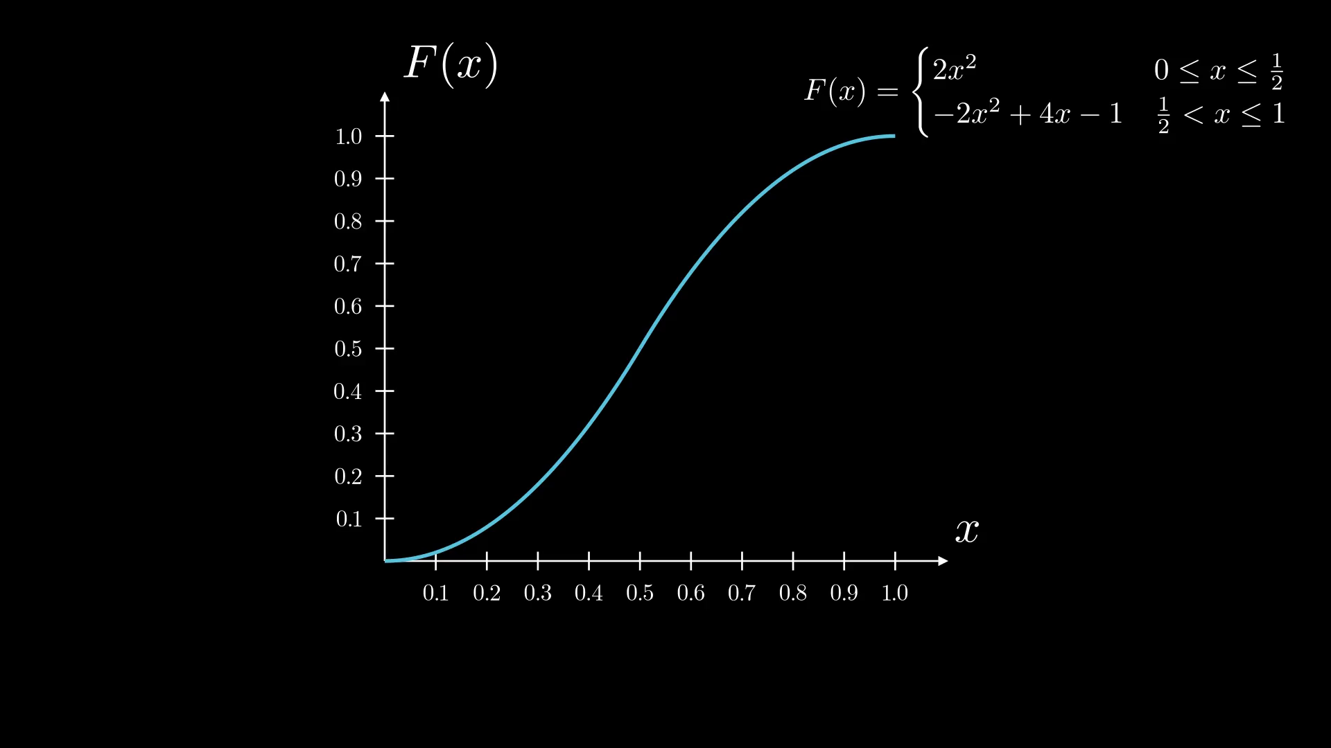
2. Next, we invert this (Figure-6)

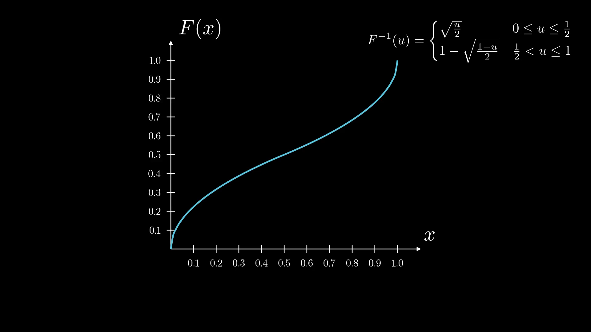
3. Now, we get a uniformly distributed sample $\xi_i$
4. Finally, we can generate $X_i = P^{-1}(\xi_i)$

This follows the desired distribution. The four steps are also visualized in Figure-7

Now, mathematically proving that this follows the PDF requires a bit more knowledge about the change of variables formula, that I intend to discuss in the future. It is far easier to see that it does indeed follow the desired distribution in the discrete case, where we know the pmf $p(x)$, lets look at an example of that next.

A Discrete PMF

In the discrete case, we don’t find the CDF by integration, rather we find it by simple summation of the probabilities - $P(x) = \sum_{0}^{x} p(x)$. The rest of the algorithm continues as described previously. So, let’s take an example and follow the algorithm-

Let’s use the pmf - $p(x)$ (Figure-8).

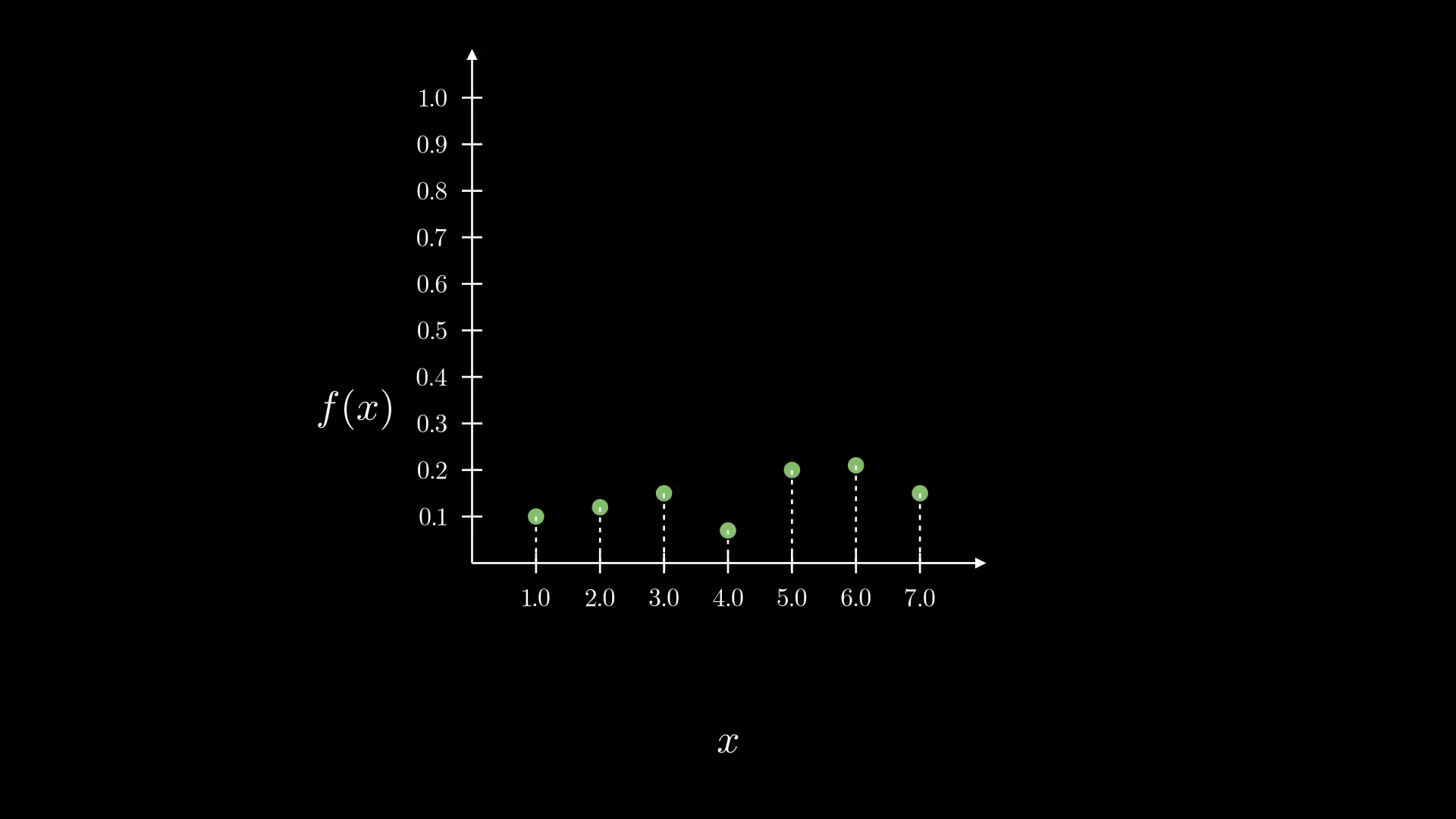
1. First, we find it’s CMF (Figure-9)

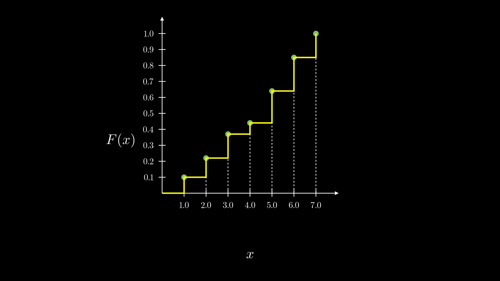
The next few steps are easily understood visually, and involve many piecewise functions, so I will explain with images rather than equations.

2. Next, we invert the CMF, Figure-10. Note that inverting a 1D function graphically is the same as flipping it around the line y = x.

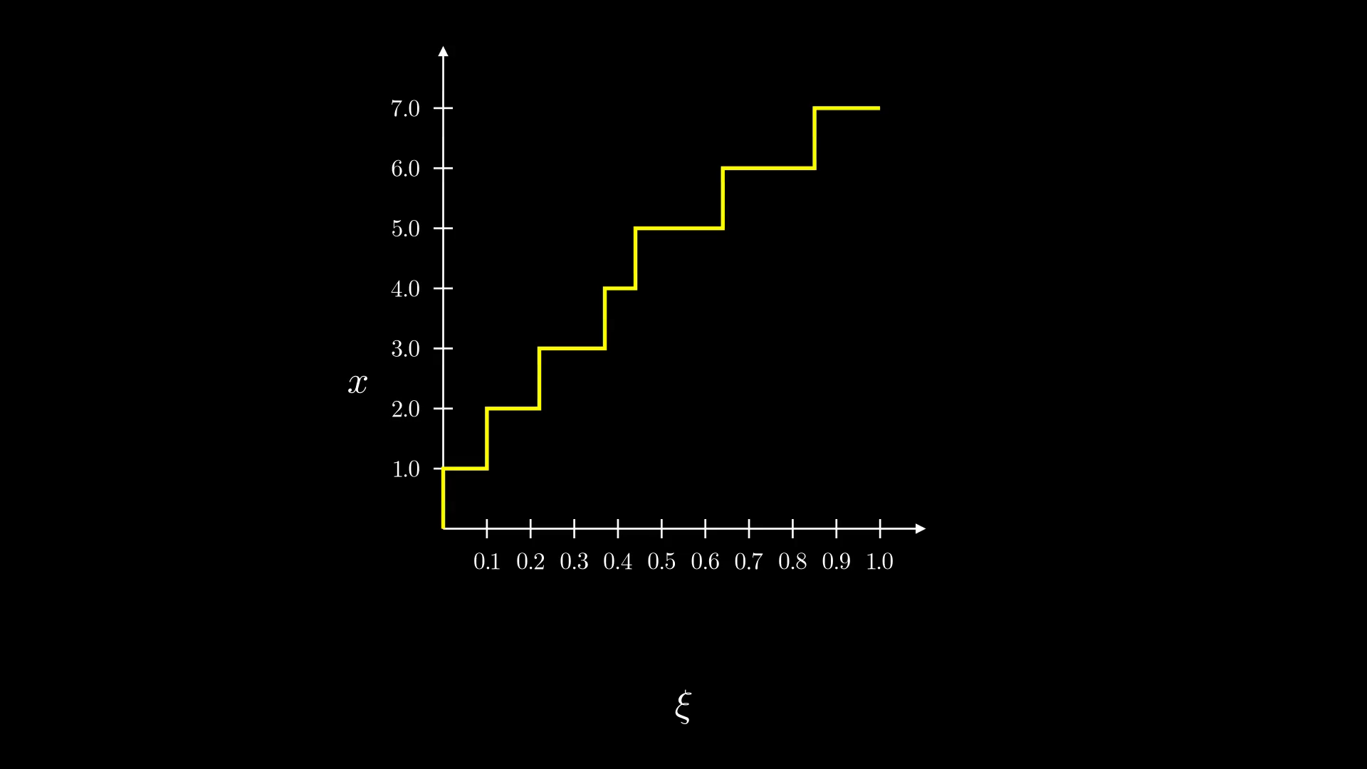
3. Now, we get a uniformly distributed sample $\xi_i$

4. Finally, we sample using $\xi_i$.

Again, these steps are visualized in Figure-11

Now, if we were to calculate the probability of getting each of the discrete numbers we clearly get -

Since that is the length of the segments corresponding to each of the discrete numbers, ($p(x)$) divided by the total lengths ($1.0$). So, we can see that the discrete case does follow our desired pmf.

Conclusion

This algorithm is quite clean, and a closed solution to generating samples. Using it we can generate random samples as we desire, but unfortunately, this method also requires that we can integrate the pdf as required, or summate the pmf without numerical instability in the case of very small probabilities. But other than this one pitfall, I think its a beautiful algorithm.

The moment I saw the visualizaation of the discrete case, the algorithm clicked for me. It seemed so simple and so elegant. I think it might just be my favorite algorithm because of that moment. I have learnt this concept in relation to pathtracers, which generally use millions or billions of random samples to generate outputs ^{4 5 6}, pathtracers are something I will hopefully write more about in the future.

I hope a bit of my passion got through to you! See you again sometime ;)