How to find the value of an un-integrable integral: Monte Carlo Integration [md]

Created: Sun Jul 12 2026

Introduction

Imagine, for a second, an arbitrary function $f(x)$ . We don’t have access to $f(x)$ or its parameters themselves, but given an input $a$ , we can get the value of $f(a)$ . A blackbox, so to speak. Now, how can one integrate $\int_a^b{f(x)}\,dx$ ? Monte Carlo Integration is one way to numerically ¹ solve this problem. But what is Monte Carlo Integration in the first place?

The Law of Large Numbers

First, lets look at a mathematical law that induces our method - the law of large numbers states that given samples of a function from independent and identically distributed values, the sample mean converges to the true mean (or true value). That is,

\lim_{N \to \infty} \frac{1}{N} \sum_{i=1}^{N} f(x_i) = \mathbb{E}[f(x)]

Now this might sound a bit confusing, so let’s consider an example, take

\begin{align} f(x|\mu, \sigma) &= \mathcal{N}(\mu, \sigma) \\ &= \frac{1}{\sqrt{2\pi\sigma^2}}exp({\frac{-(x-\mu)^2}{2\sigma^2}}) \end{align}

that is, a normal distribution centered on $x = \mu$ with a standard deviation of $\sigma$ . The true mean of the function is $\mu$ . Now, the law of large numbers states that, given $N$ independent (obtaining a random number does not affect obtaining the next one) and identically distributed (all are obtained from the same distribution) samples $x_1...x_N$ ², that

\lim_{N \to \infty} \frac{1}{N} \sum_{i=1}^{N} f(x_i) = \mu

In the widget, you can perform a monte carlo simulation. Note that as we generate more samples, the sample mean converges to the true mean. I will expand on this more below.

That is, if we find the average of infinite random samples of the function $f(x)$ , we will obtain the true mean, $\mu$ . Note that this can be accomplished even if the function is a blackbox, since we only need the ability to find the value of the function at random points, no access to the parameters themselves.

Towards Monte Carlo Integration

Now, once again, let’s look at the function $Y = f(x)$ . Lets say we define a probability domain $p(x)$ for each $x$ . Then, we can find the expected value of this function as -

\mathbb{E}[Y] = \int_D f(x)p(x) \,dx

Where $D$ is the domain of $x$ (For example, if $x$ is a random number between $0$ and $1$ , then $D = [0, 1]$ ).

But we know from the law of large numbers that

\mathbb{E}[Y] \approx \frac{1}{N}\sum_{i=1}^N f(x_i)

So, we can see that

\int_D f(x)p(x) \,dx \approx \frac{1}{N}\sum_{i=1}^N f(x_i)

Now, consider another function, that we define as

g(x) = \frac{f(x)}{p(x)}

Then, we can once again say that

\begin{align} \int_D g(x)p(x) \,dx &\approx \frac{1}{N}\sum_{i=1}^N g(x_i) \\ \int_D \frac{f(x)}{p(x)}p(x) \,dx &\approx \frac{1}{N}\sum_{i=1}^N \frac{f(x_i)}{p(x_i)} \\ \int_D \frac{f(x)}{\cancel{p(x)}}\cancel{p(x)} \,dx &\approx \frac{1}{N}\sum_{i=1}^N \frac{f(x_i)}{p(x_i)} \\ \int_D f(x) \,dx &\approx \frac{1}{N}\sum_{i=1}^N \frac{f(x_i)}{p(x_i)} \\ \end{align}

So, we can find the value of the integral we wanted, simply by sampling the function at a large number of points.

An example of Monte Carlo Integration

Let’s once again look at an example to understand this better. Let’s attempt to find the area under the graph $e^{sin(3x^2)}$ , between $x=a$ and $x=b$ . That is, we want to find -

I = \int_a^b e^{sin(3x^2)} \, dx

First, we must select a pdf for $x_i$ . Lets choose the uniform distribution, since our domain is $[a, b]$ ,

p(x) = \frac{1}{b-a}

From our derivation, we have

\begin{align} I &= \int_a^b e^{sin(3x^2)} \, dx \\ \int_a^b e^{sin(3x^2)} \, dx &\approx \frac{1}{N} \sum_{i=1}^N \frac{e^{sin(3x_i^2)}}{p(x_i)} \\ &\approx \frac{1}{N} \sum_{i=1}^N \frac{e^{sin(3x_i^2)}}{\frac{1}{b-a}} \\ &\approx \frac{1}{N} \sum_{i=1}^N \frac{e^{sin(3x_i^2)\cdot(b-a)}}{1} \\ &\approx \frac{1}{N} \sum_{i=1}^N e^{sin(3x_i^2)} \cdot (b-a) \\ &\approx \frac{b-a}{N} \sum_{i=1}^N e^{sin(3x_i^2)} \\ \end{align}

Lets try to take a few samples, and understand what this means graphically. Here, I have set $a=0$ and $b=1$ . Next, I took 4 samples and plotted the value of the function at those samples. If you note the second-to-last equation, you will see that we are calculating

\begin{align} I &\approx \frac{1}{N} \sum_{i=1}^N e^{sin(3x_i^2)} \cdot (b-a) \\ &\approx \frac{1}{N} \sum_{i=1}^N f(x) \cdot (b-a) \\ \end{align}

This is merely the averagea of the areas of all rectangles with base $b-a$ and height $f(x_i)$ for all our samples. This is easier visualized in Figure-1.

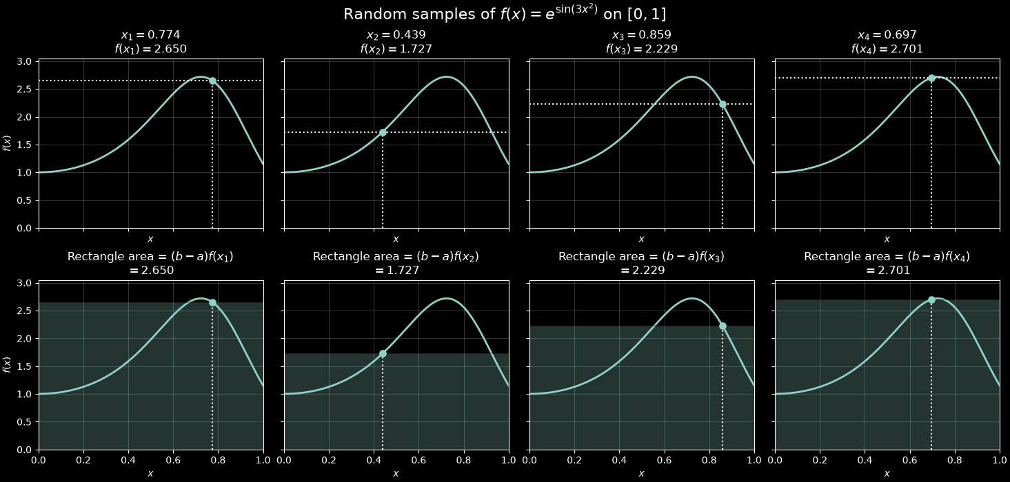
Figure 1: A visualization of Monte Carlo Integration, with 4 samples. The first row shows the values of the 4 samples. The second row shows the 4 rectangles created by the common base, and the values of the samples

This means that, if we average the areas of the rectangles subtended by an infinite number of samples, we will approach the true value of the integral. But what is the benefit to using this technique? The answer lies in how this approximation approaches the true value of the integral.

Convergence, or, why we need a large number of samples

Now, we have established previously, that from the law of large numbers, we can derive that -

\int_D f(x) \,dx \approx \frac{1}{N}\sum_{i=1}^N \frac{f(x_i)}{p(x_i)}

But note the $\approx$ instead of a $=$ . So, how much can we trust this estimate of the integral?

First, we need to discuss some things about functions that rely on randomness. If you are familiar with probability theory, you would be familiar with $V$ , the variance of a random variable. This is a measure that dictates how much a random variable “deviates from the norm” - how all-over the place it is. Now, this measure is defined as -

V[f(x)] = \mathbb{E}[(f(x) - \mathbb{E}[f(x)])^2]

That is, its the average squared error of the function. This measure has 2 properties we will use in our further proofs -

V[af(x)] = a^2V[f(x)]

where $a$ is any scalar constant, and

V[f(x) + g(x)] = V[f(x)] + V[g(x)]

where $f(x)$ and $g(x)$ are independent functions.

Now, we can define how much trust we have in our estimate of the integral by finding out its variance - the lower the variance, the closer it is to the true value, and vice versa. Lets find this value -

we want to find

\begin{align} V \left[ \frac{1}{N}\sum_{i=1}^N \frac{f(x_i)}{p(x_i)} \right] &= \frac{1}{N^2} V \left[ \sum_{i=1}^N \frac{f(x_i)}{p(x_i)} \right] \end{align}

This derives from the first rule about variance we discussed above, next -

\begin{align} V \left[ \frac{1}{N}\sum_{i=1}^N \frac{f(x_i)}{p(x_i)} \right] &= \frac{1}{N^2} V \left[ \sum_{i=1}^N \frac{f(x_i)}{p(x_i)} \right] \\ &= \frac{1}{N^2} \sum_{i=1}^N V \left[ \frac{f(x_i)}{p(x_i)} \right] \end{align}

This derives from the second rule discussed above, since $f(x)$ is independent (does not depend on previous values of itself), and since $p(x)$ is also independent. Finally, we can say that since for any given $x_i$ , $f(x_i)$ and $p(x_i)$ are identical (not numerically), but since $x_i$ are all drawn from the same distribution, so the randomness only depends on $x_i$ , we can say that the variance of all $i$ samples, would be the same, so we can claim that -

\begin{align} V \left[ \frac{1}{N}\sum_{i=1}^N \frac{f(x_i)}{p(x_i)} \right] &= \frac{1}{N^2} V \left[ \sum_{i=1}^N \frac{f(x_i)}{p(x_i)} \right] \\ &= \frac{1}{N^2} \sum_{i=1}^N V \left[ \frac{f(x_i)}{p(x_i)} \right] \\ &= \frac{1}{N^2} N \cdot \left( V \left[ \frac{f(x)}{p(x)} \right] \right) \\ &= \frac{1}{N} \cdot \left( V \left[ \frac{f(x)}{p(x)} \right] \right) \\ &= \frac{1}{N} \cdot \left( \text{Variance of 1 sample} \right) \\ &\propto \frac{1}{N} \end{align}

So, as we can see, the variance of our estimate, $V$ is proportional to $\frac{1}{N}$ . This means that if we increase our number of samples, it makes our estimate better.

This is also true intuitively, as in the case discussed above of finding the true mean of a normal distribution, as we generate more samples, we get closer and closer to the average becoming the true mean, $\mu$ .

Once again, this may be better understood visually, lets look at an example.

Visualizing the efficacy of a Monte Carlo Method

Let’s look at a function that we can integrate easily -

I = \int_{-\frac{\pi}{2}}^{\frac{\pi}{2}} cosx \, dx

First, lets find the answer analytically -

\begin{align} I &= \int_{-\frac{\pi}{2}}^{\frac{\pi}{2}} cosx \, dx \\ \int_{-\frac{\pi}{2}}^{\frac{\pi}{2}} cosx \, dx &= \left[ sinx \right]_{-\frac{\pi}{2}}^{{\frac{\pi}{2}}} \\ &= [sin(\frac{\pi}{2}) - sin(-\frac{\pi}{2})] \\ &= [1 - (-1)] \\ &= 2 \end{align}

Now, lets apply the monte carlo method.

First, we take a probability distribution,

\begin{align} p(x) &= \frac{1}{\frac{\pi}{2} - (-\frac{\pi}{2})} &= \frac{1}{\pi} \end{align}

Now, Lets sample using this probability distribution and use monte carlo integration -

\begin{align} I &\approx \frac{1}{N} \sum_{i=1}^{N} \frac{f(x_i)}{p(x_i)} \\ &\approx \frac{1}{N} \sum_{i=1}^{N} \frac{cos(x_i)}{\frac{1}{\pi}} \\ &\approx \frac{1}{N} \sum_{i=1}^{N} \pi cos(x_i) \\ \end{align}

Lets do this, and plot it out, as well as the resulting variance. In the widget below, the graph on top plots the estimate of the integral, overlaid on the true value. The bottom graph plots the variance of the estimation.

Clearly, the estimate approximates the true value, $2$ . Furthermore, the estimate variance also drops, following the rule of $V \propto \frac{1}{N}$ .

Conclusion

As we can see, using Monte Carlo Integration, we can solve integrals numerically that are impossible to solve analytically, such as $\int e^{x^2} \,dx$ . It is extremely powerful, and find many uses. While I did not entirely explain exactly what the Monte Carlo method is (and it’s alternatives), I hope you understood what Monte Carlo Integration is.

The Monte Carlo method induces many algorithms that make use of random numbers. Monte Carlo integration is just one of them. While it might seem a bit abstract to introduce these now, Monte Carlo integration is the core algorithm used in all path tracers³. Using computers capable of processing millions of samples in a second, it is plain to see that Monte Carlo Integration can be extensively used.

I personally like the elegance of understanding monte carlo integration simply to be averaging the areas of rectangles subtended by random samples, and that is why I wrote this article about it. I also intend to continue these articles until I satisfactorily explain how they are relevant to pathtracing.

to approximate the integral $\int_{a}^{b}{f(x)}\,dx$ to a given degree of accuracy, with a given $a$ and $b$ . ↩
In this article, we assume that it is possible to obtain uniformly distributed samples between a given range (usually $[0, 1]$ ). I.e., it is possible to obtain samples that all have the same probability. ↩
https://en.wikipedia.org/wiki/Path_tracing ↩